| 일 | 월 | 화 | 수 | 목 | 금 | 토 |
|---|---|---|---|---|---|---|
| 1 | 2 | 3 | 4 | 5 | ||
| 6 | 7 | 8 | 9 | 10 | 11 | 12 |
| 13 | 14 | 15 | 16 | 17 | 18 | 19 |
| 20 | 21 | 22 | 23 | 24 | 25 | 26 |
| 27 | 28 | 29 | 30 |
- 언리얼엔진
- cv
- motion matching
- GAN
- 생성모델
- 폰트생성
- WBP
- ddpm
- Few-shot generation
- BERT
- 모션매칭
- ue5.4
- dl
- WinAPI
- NLP
- CNN
- multimodal
- Generative Model
- 디퓨전모델
- UE5
- 딥러닝
- Unreal Engine
- userwidget
- deep learning
- Diffusion
- animation retargeting
- RNN
- Font Generation
- Stat110
- 오블완
- Today
- Total
Deeper Learning
DDPM: Denoising Diffusion Probabilistic Models 본문
Jonathan Ho, Ajay Jain, Pieter Abbeel, (2020.06) [UC Berkeley]
[이후 Cold Diffusion 논문에서 Gaussian Noise가 아닌 다른 Noise를 사용하여 학습이 가능함을 보였기 때문에, 해당 파트에 대한 수식은 간단하게 다룸, Langevin dynamics 또한 다루지 않음]
Abstract
- 비평형 열역학에서 영감을 받은 latent variable model인 diffusion 확률 모델을 사용한 고품질의 이미지 생성 방법론을 제시
- diffusion 확률 모델, denoising score matching, Langevin dynamics의 관계를 활용하여 디자인한 weighted variational bound로 학습
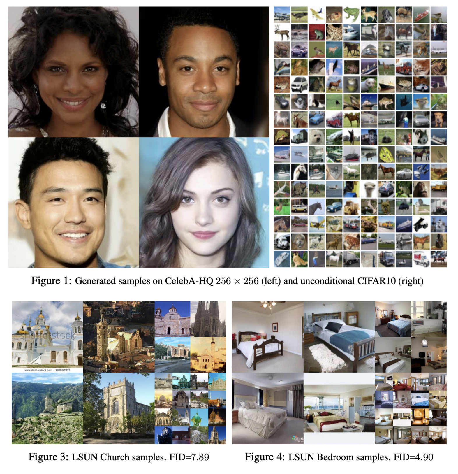
- CIFAR-10 unconditional generation에서 FID SOTA 달성, LSUN에서도 ProgressiveGAN과 비슷한 성능을 보임
1. Introduction

- VAE, GAN, AR models, flows, energy-based modeling, score matching 등 여러 이미지 생성 방법론이 연구되어 왔음
- 본 논문은 diffusion 확률 모델을 개선한 것, diffusion 확률 모델은 variational inference를 사용하여 학습하는 parameterized Markov chain
- noise를 제거하는 Markov chain denoise를 학습
- diffusion 모델은 학습이 효율적이나 고품질의 생성을 할 수 있는지는 이전에 알 수 없었음. 본 논문에서 제시
2. Background
- predicted mu, sigma로 Gaussian distribution을 만들고 이를 활용하여 이미지를 denoise
- 다른 모델들과 다른 diffusion 모델의 큰 특징은 approximate posterior q(xi:T|x0)가 Gaussian noise를 연속적으로 더하는 Markov chain인 diffusion process(forward process)로 고정되어 있다는 것 (식(2), β 는 variance schedule)
- joint distribution pθ(x0:T)는 reverse process라고 부르며 p(xT)=N(xT;0,I) 에서 시작하는 학습된 Gaussian transition으로 구성된 Markov chain으로 정의되어 있다. (식(1))
- 즉, forward process, reverse process 모두 한 step이 Gaussian process로 구성된 Markov Chain
수식을 보기 전에 Diffusion 개념 코드와 함께 정리
실제로 코드상에서 Diffusion 모델의 학습은 다음과 같이 이루어진다.
- 임의의 timestep을 선정
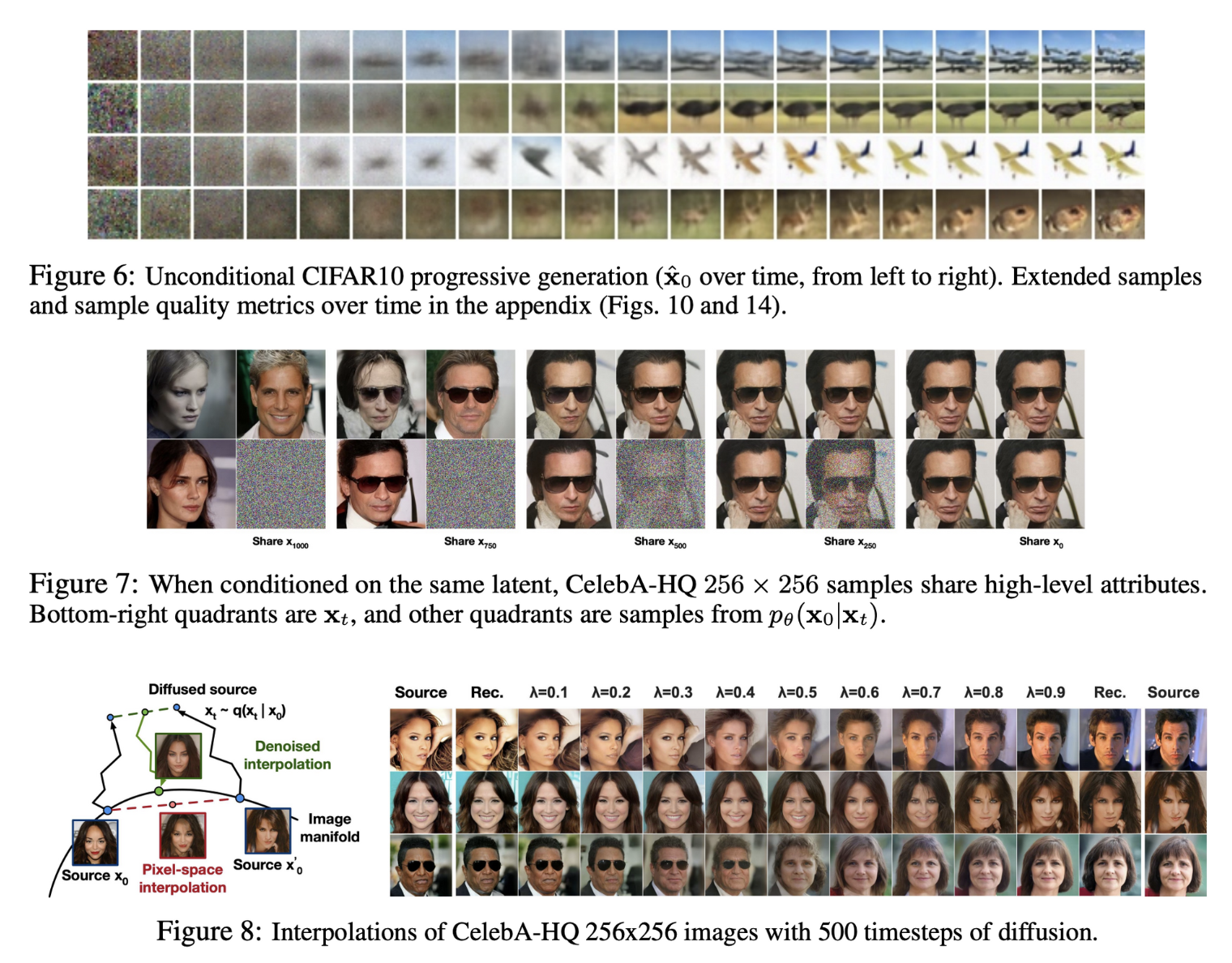
- 시작 원본 이미지에서 해당 timestep까지의 forward process를 적용한 이미지와 해당 time step +1 까지의 forward process를 적용한 이미지를 만듦
- 두 이미지 사이의 denoise process를 학습
- noise와의 L1 or L2 loss 사용
원본 이미지에서 바로 900 timestep의 forward process가 적용된 이미지를 위 (2) 식에서 β 를 이용하여 얻으려면 병렬처리가 불가능한 노이즈를 순차적으로 적용해야 하는 문제가 있다.
αt=1−βt,ˉαt=t∏s=1αsq(xt|x0)=N(xt;√ˉαtx0;(1−ˉαtI)
위 수식을 이용하면 한 번에 임의의 timestep의 forward process가 적용된 결과를 한 번에 얻을 수 있다. 미리 alpha를 모두 계산해 두고 요구하는 time step에 맞는 index의 값을 가져와 바로 사용
# q_sample code snippet
# from <https://github.com/lucidrains/denoising-diffusion-pytorch>

alphas_cumprod = torch.cumprod(alphas, dim=0)
def q_sample(self, x_start, t, noise=None):
        noise = default(noise, lambda: torch.randn_like(x_start))

        return (
            extract(self.sqrt_alphas_cumprod, t, x_start.shape) * x_start +
            extract(self.sqrt_one_minus_alphas_cumprod, t, x_start.shape) * noise
        )
# p_losses code snippet
# from <https://github.com/lucidrains/denoising-diffusion-pytorch>

def forward(self, img, *args, **kwargs):
        b, c, h, w, device, img_size, = *img.shape, img.device, self.image_size
        assert h == img_size and w == img_size, f'height and width of image must be {img_size}'
        t = torch.randint(0, self.num_timesteps, (b,), device=device).long()

        img = normalize_to_neg_one_to_one(img)
        # print(img.max(), img.min())
        return self.p_losses(img, t, *args, **kwargs)

def p_losses(self, x_start, t, noise = None):
        b, c, h, w = x_start.shape
        noise = default(noise, lambda: torch.randn_like(x_start))

        # noise sample

        x = self.q_sample(x_start = x_start, t = t, noise = noise)

        # if doing self-conditioning, 50% of the time, predict x_start from current set of times
        # and condition with unet with that
        # this technique will slow down training by 25%, but seems to lower FID significantly

        x_self_cond = None
        if self.self_condition and random() < 0.5:
            with torch.no_grad():
                x_self_cond = self.model_predictions(x, t).pred_x_start
                x_self_cond.detach_()

        # predict and take gradient step

        model_out = self.model(x, t, x_self_cond)

        if self.objective == 'pred_noise':
            target = noise
        elif self.objective == 'pred_x0':
            target = x_start
        elif self.objective == 'pred_v':
            v = self.predict_v(x_start, t, noise)
            target = v
        else:
            raise ValueError(f'unknown objective {self.objective}')

        loss = self.loss_fn(model_out, target, reduction = 'none')
        loss = reduce(loss, 'b ... -> b (...)', 'mean')

        loss = loss * extract(self.p2_loss_weight, t, loss.shape)
        return loss.mean()
학습 과정은 결국 Gaussian noise를 step마다 적용하는 forward process를 reverse 할 수 있도록 하는 parameterized model을 학습하는 것
코드상 동작은 Noise를 예측하고 Noise와의 L1 or L2 loss를 통해 UNet을 학습, 그렇게 예측한 noise를 가지고 아래 식을 통해 image를 denoise (Noise→Image 때 사용)
# pseudo code

def p_loss():
  noise = torch.randn_like(x_start)
	pred_noise = model.forward(x, t)
	loss = l1_loss(noise, pred_noise)


def predict_start_from_noise(self, x_t, t, noise):
        return (
            extract(self.sqrt_recip_alphas_cumprod, t, x_t.shape) * x_t -
            extract(self.sqrt_recipm1_alphas_cumprod, t, x_t.shape) * noise
        )
Forward, Reverse Process에 대한 설명을 마치고 Reverse Process를 어떻게 학습할지에 대해서 알아보겠다.
3. Diffusion models and denoising autoencoders
VAE와 DDPM의 수식 유도 과정은 MLE objective, ELBO, intractable term의 제거 등 전개 과정이 유사하다.
term을 맞추기 위해 VAE에서도 z대신 xT사용
수식전개 출처: (https://developers-shack.tistory.com/8)
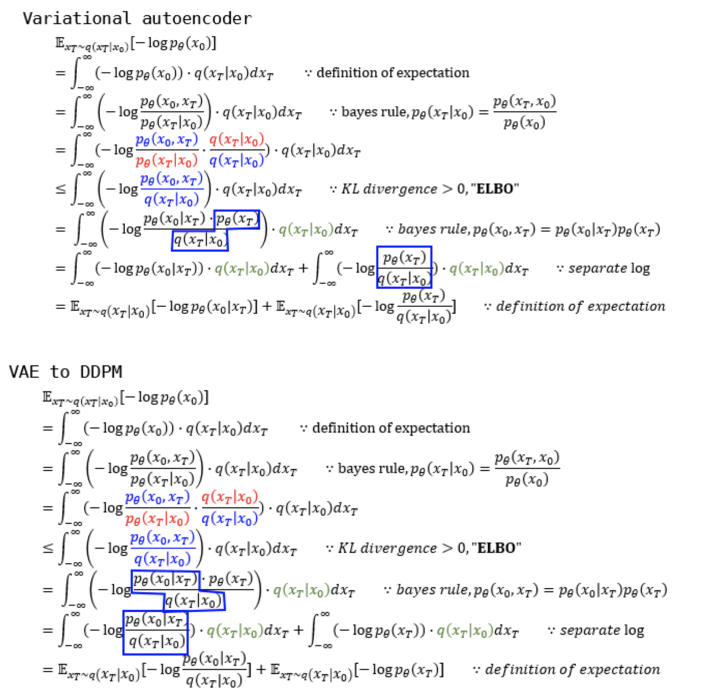
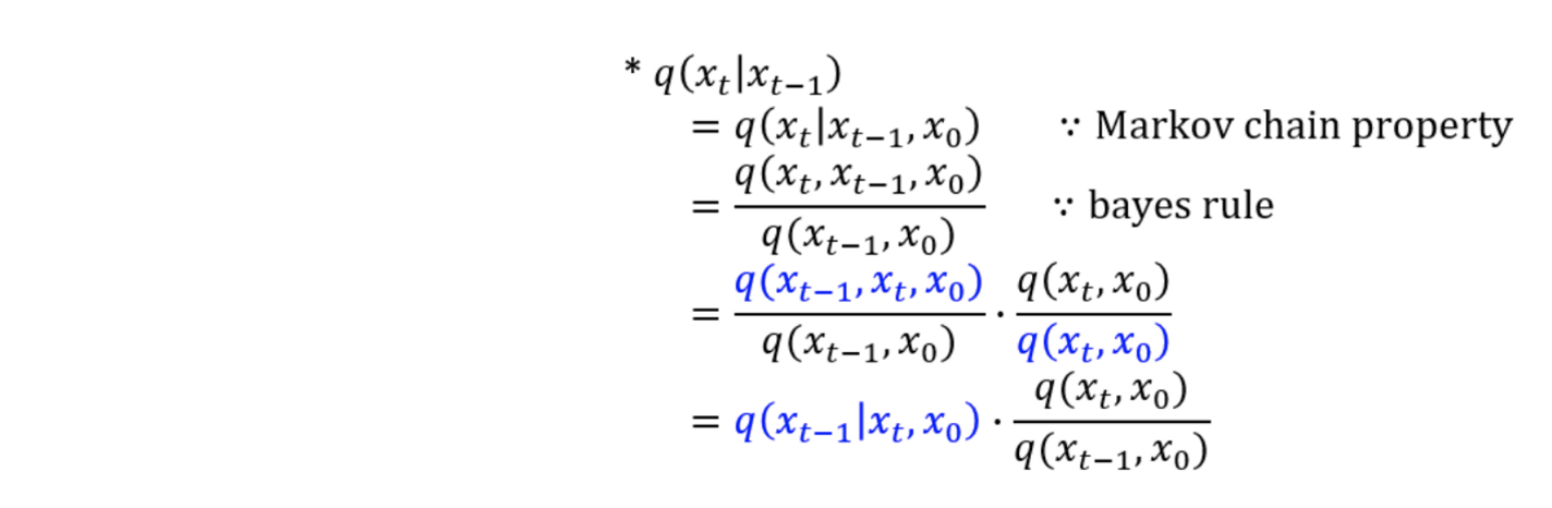
reverse process는 forward process를 활용하여 학습이 되어야 하는데 위의 DDPM 전개식의 마지막 줄의 첫째 항을 보면 condition과 target이 서로 다른 pθ(x0|xt),q(xT|x0)의 KL-divergence가 loss로 주어진다.
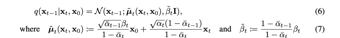
single reverse process pθ(xt−1|xt)가 tractable한 single forward process q(xt−1|xt,x0)와 KL divergence로 직접 비교할 수 있도록 식을 다시 세워보자. (수식 (6,7) 참고)
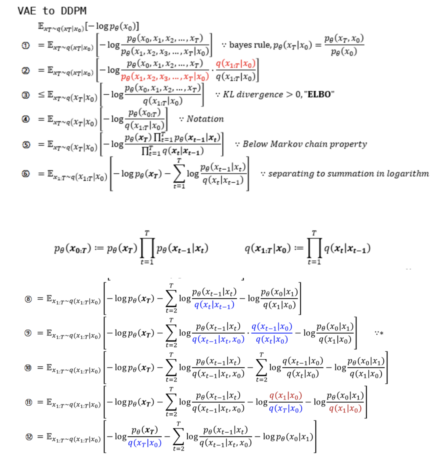
전개한 최종 loss 식을 KL divergence 형태로 바꿔 표현하면 아래와 같다.
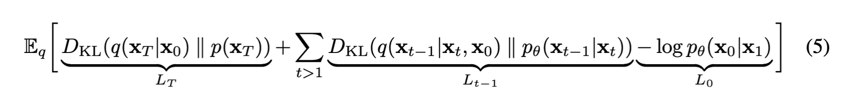
LT는 forward process를 통해 얻은 Noise q(xT|x0)과 p(xT)의 KL divergence인데 저자는 forward process의 학습 가능한 parameter βt를 상수로 고정하였기 때문에 learnable parameter가 없어 학습에 사용되지 않고 무시되는 term이다.
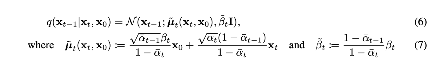
Lt−1: pθ(xt−1|xt)은 parameter set θ로 구성된 parameterized model이 μ,σ를 추정하여 만드는 분포로 N(xt−1;μθ(xt,t),Σθ(xt,t))로 식을 쓸 수 있다. 저자는 Σθ(xt,t)를 time에 따라 결정되는 고정 상수 σ2I로 고정하였다. forward process도 위 수식(6,7)을 사용하여 나타내면 Lt−1은 아래와 같이 다시 쓸 수 있다.
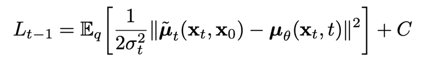
결국 Lt−1은 forward process의 posterior mean ˜μt을 추정하는 것과 같다.
VAE와 비슷하게 reparameterization trick을 통해 식을 다시 쓰면

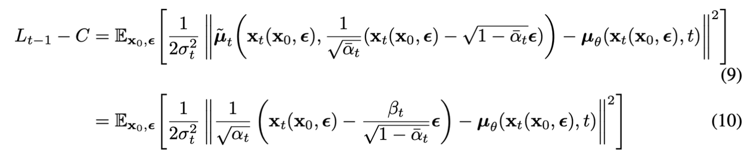
(10)식을 보면 μθ는 주어진 xt에서 1√αt(xt−βt√1−ˉαtϵ)를 예측해야 한다.
xt는 모델의 input으로 사용가능하기 때문에, xt로 parameterization하면

ϵθ는 xt,t를 사용하여 표준 가우시안 노이즈 ϵ를 추정
즉, xt−1∼pθ(xt−1|xt)를 샘플링하는 것은 xt−1=1√αt(xt−βt√1−ˉαtϵθ(xt,t))+σtz를 계산하는 것과 같다.
식 (10)도 식(11)을 사용하여 간단하게 정리하면 아래식과 같다.
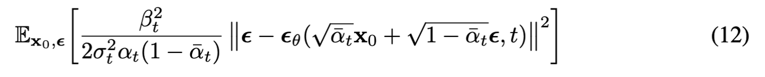
식(12)의 앞 계수를 1로 설정하였을 때, 실험결과가 더 좋았음.
training, sampling 식을 정리하면 아래 표와 같다.
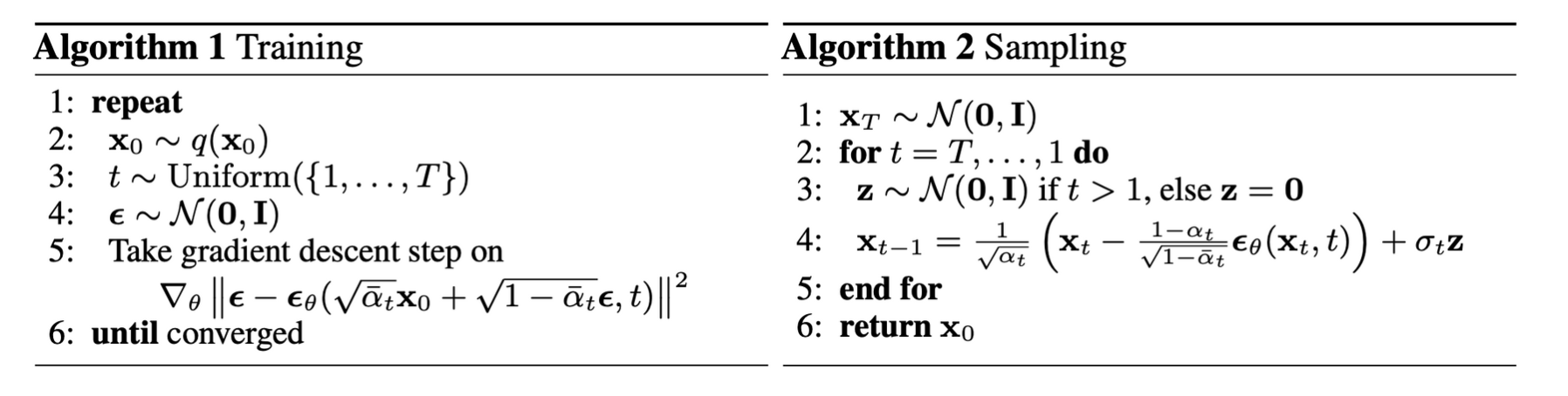
요악하면
- reverse process를 mean function approximator μθ를 forward process의 posterior mean ˜μt를 예측하도록 학습할 수 있다
- reparameterization trick을 사용하여 ϵ을 추정하도록 학습할 수도 있음. (Langevin dynamics, denoising score matching
- x0을 추정하도록 학습시킬 수도 있으나 성능이 좋지 않았음.
L0은 원본 이미지 x0를 x1에 reverse process를 적용하여 추정하는 term
Simplified training objective
LT는 학습에서 제외하고 Lt−1,L0를 하나로 묶어(몇 가지 근사, 가정이 추가) MSE 형태로 간단하게 만들 수 있다.

위 loss는 매우 작은 noise를 denoise 하기 때문에 model weight의 크기를 줄이는데 효율적
4. Experiments
- Parameters는 shared across time, sinusoidal position embedding을 사용
- GroupNorm, low-resolution에서 self-attention 사용
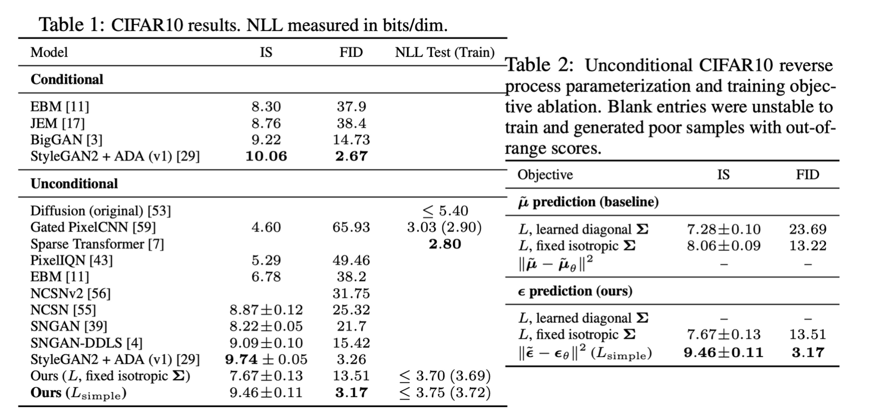
- CIFAR 10 unconditional generation에서 뛰어난 성능을 보임
- ˜μ prediction은 단순화한 loss인 MSE에서는 작동하지 않았으며, $\epsilon$ prediction은 MSE와 함께 사용하면 좋은 퀄리티의 샘플을 생성
5. Conclusion
- Diffusion을 사용하여 고품질의 이미지 생성에 성공
- Diffusion model과 Markov chain 학습을 위한 variational inference, denoising score matching과 Langevin dynamics, autoregressive model과 progressive lossy compression의 연결점을 찾음
- Diffusion 모델은 image 데이터에 대해 뛰어난 inductive bias를 가지고 있는 것으로 보이기 때문에 다른 modalities, 머신러닝 시스템에서 다른 생성 모델의 components로 사용 등 후속 연구를 제시
후기&정리
- Diffusion 모델을 사용하여 고품질의 이미지 생성 성공
- text-to-image, inpainting 등 여러 현재(2023.01) image generative model에서 사용하는 base training method인 diffusion model의 연구를 점화시킨 논문
- 여러 실험 데이터셋으로 직접 학습시켜 보니 모델 구조가 간단하고(U-Net) 모든 timestep에서 같은 weight를 share 하기 때문에 모델이 가볍고 MLE objective이기 때문에 GAN 보다 학습 또한 쉽고 강건하였음.
- 후에 나온 논문인 Cold-diffusion에서는 Gaussian noise를 사용하지 않고 diffusion의 학습에 성공
- DDPM의 성공은 Gaussian noise를 사용하였기 때문에 전개 가능한 수식으로 얻은 loss 뿐만 아니라 다른 요소에서 오는 이점이 존재한다는 증거
- 으레 그렇듯 논문에서 제시한 실험을 통해 경험적으로 사용하는 loss, 여러 trick들이 후에 나온 다른 논문에 의해 대체될 것이라고 생각
Reference
[0] Jonathan Ho et al. (2020). "Denoising Diffusion Probabilistic Models". https://arxiv.org/abs/2006.11239
Denoising Diffusion Probabilistic Models
We present high quality image synthesis results using diffusion probabilistic models, a class of latent variable models inspired by considerations from nonequilibrium thermodynamics. Our best results are obtained by training on a weighted variational bound
arxiv.org
[1] https://github.com/lucidrains/denoising-diffusion-pytorch
GitHub - lucidrains/denoising-diffusion-pytorch: Implementation of Denoising Diffusion Probabilistic Model in Pytorch
Implementation of Denoising Diffusion Probabilistic Model in Pytorch - GitHub - lucidrains/denoising-diffusion-pytorch: Implementation of Denoising Diffusion Probabilistic Model in Pytorch
github.com
[2] Arbit Bansal et al. (2022). "Cold Diffusion: Inverting Arbitrary Image Transforms Without Noise". https://arxiv.org/abs/2208.09392
Cold Diffusion: Inverting Arbitrary Image Transforms Without Noise
Standard diffusion models involve an image transform -- adding Gaussian noise -- and an image restoration operator that inverts this degradation. We observe that the generative behavior of diffusion models is not strongly dependent on the choice of image d
arxiv.org
[3] https://developers-shack.tistory.com/8
[논문공부] Denoising Diffusion Probabilistic Models (DDPM) 설명
─ 들어가며 ─ 심심할때마다 아카이브에서 머신러닝 카테고리에서 그날 올라온 논문들이랑 paperswithcode를 봅니다. 아카이브 추세나 ICLR, ICML 등 주변 지인들 학회 쓰는거 보니까 이번 상반기에
developers-shack.tistory.com
'AI > Deep Learning' 카테고리의 다른 글
| DDIM: Denoising Diffusion Implicit Models (0) | 2023.04.14 |
|---|---|
| Diffusion Model 수식 정리 (0) | 2023.04.08 |
| SGCE-Font: Skeleton Guided Channel Expansion for Chinese Font Generation (0) | 2022.12.10 |
| StrokeGAN+: Few-Shot Semi-Supervised Chinese Font Generation with Stroke Encoding (0) | 2022.12.06 |
| Zero-Shot Text-to-Image Generation (0) | 2022.12.03 |


