| 일 | 월 | 화 | 수 | 목 | 금 | 토 |
|---|---|---|---|---|---|---|
| 1 | 2 | 3 | 4 | 5 | 6 | 7 |
| 8 | 9 | 10 | 11 | 12 | 13 | 14 |
| 15 | 16 | 17 | 18 | 19 | 20 | 21 |
| 22 | 23 | 24 | 25 | 26 | 27 | 28 |
| 29 | 30 | 31 |
- 폰트생성
- UE5
- RNN
- 생성모델
- Unreal Engine
- 오블완
- dl
- 모션매칭
- animation retargeting
- Font Generation
- Few-shot generation
- ddpm
- userwidget
- 언리얼엔진
- Generative Model
- multimodal
- 디퓨전모델
- 딥러닝
- Diffusion
- WBP
- Stat110
- cv
- motion matching
- CNN
- ue5.4
- WinAPI
- deep learning
- GAN
- BERT
- NLP
- Today
- Total
Deeper Learning
Score-Based Generative Modeling through Stochastic Differential Equations 본문
Score-Based Generative Modeling through Stochastic Differential Equations
Dlaiml 2023. 5. 27. 21:24Yang Song, Jascha Sohl-Dickstein, Diederik P. Kingma, Abhishek Kumar, Stefano Ermon, Ben Poole, (2020.11) [Stanford, Google]
Why score function?
생성모델을 학습한다는 것은 데이터 분포 $p_\theta(x)$ 를 근사하는 것과 같다. likelihood based 모델에서는 직접적으로 pmf 또는 pdf를 모델링하는데 아래 식처럼 학습가능한 parameter set $\theta$ 로 parameterize된 Real-valued function $f_\theta(x)$ 를 사용하여 pdf를 정의할 수 있다.
$$ p_\theta(x) = \frac{e^{-f_\theta}(x)}{Z_\theta} $$
여기에서 $Z_\theta$ 는 normalizing constant로 $\int_x p_\theta(x)dx$ 가 1이 되도록 하는 역할을 한다.
$f_\theta(x)$ 는 unnormalized probabilistic model, energy-based model로 불린다.
$p_\theta(x)$ 는 data의 log-likelihood를 maximize하는 방식으로 학습이 가능하다.
$$ \max_\theta \Sigma_{i=1}^N\log p_\theta(x_i) $$
문제는 이를 계산하기 위해서는 보통 intractable한 $Z_\theta$ 를 다루어야 한다는 것이다. 이를 해결하기 위해 likelihood-based 모델 프레임워크에서는 모델의 아키텍처를 제한하거나 (autoregressive models의 causal covolution, normalizing flow의 invertible network) normalizing constant를 근사하는 방식(VAE의 variational inference, contrastive divergence의 MCMC sampling)을 택했다.
score function은 $\nabla_x\log p(x)$ 로 정의되는데 score function을 근사하기 위한 모델을 score-based model이라고 부른다.
$$ s_\theta(x) \approx \nabla_x\log p(x) $$
score-based 모델의 큰 장점은 $x$ 에 대한 미분을 하기 때문에 생기는데 아래 식을 보면 normalizing constant의 $x$ 에 대한 미분값이 0이 되어 intractable한 normalizing constant에 대한 걱정이 사라지게 된다.
$$ s_\theta(x) = \nabla_x \log p_\theta(x) = -\nabla_xf_\theta(x) - \nabla_x\log Z_\theta = -\nabla_xf_\theta(x) $$
이제 normalizing constant를 tractable하게 하도록 특정 모델 아키텍처를 사용해야 한다는 제약에서 벗어나게 되었다.
Score Estimation

Score-based 모델의 장점에 대해서는 알게 되었는데 이제 어떻게 이를 근사할지에 대해 다뤄보자.
input, output이 같은 차원인 Score model을 통해 추정한 score function과 실제 score function의 Fisher divergence를 최소화하는 방식으로 score-based model은 학습된다.
$$ E_{p(x)}[||\nabla_x \log p(x)-s_\theta(x)||_2^2] $$
하지만 실제 score는 실제 데이터 분포의 $x$ 에 대한 편미분값으로 실제 데이터분포를 모르기 때문에 실제 score function 또한 알지 못하는 상황인데, ground-truth score function을 알지 못하는 상황에서 Fisher divergence를 minimize하는 여러 score matching 방법론이 존재한다.
Aapo Hyv¨arinen이 2005년에 제시한 score matching 방법론은 아래와 같다.
$$ E_{p_{data}}[\frac12||s_\theta(x)||^2_2+trace(\nabla_xs_\theta(x))] $$
위 score matching 식을 해석해보면 식을 최소화 한다는 것은 $||s_\theta(x)||^2_2$ 부분이 0이 되어야 하는데 이는 $x$ 에 대한 미분값이 0인 것으로 최댓값 또는 최솟값을 원한다는 것을 알 수 있으며, score function을 다시 미분하는 뒷부분은 -inf가 되었을 때 loss가 최소화되기 때문에 이는 즉, 본 함수 $p(x)$ 가 최대화되는 지점을 찾는 것과 같다는 것을 알 수 있다.
Score Estimation
Score estimation에는 문제가 하나 있는데 데이터가 부족한 영역에서는 정확한 score를 추정하기가 쉽지 않다는 것이다. 이를 완화하기 위해 data에 noise를 더하고 perturbed data에 대해 score를 추정하는 방식을 사용한다.
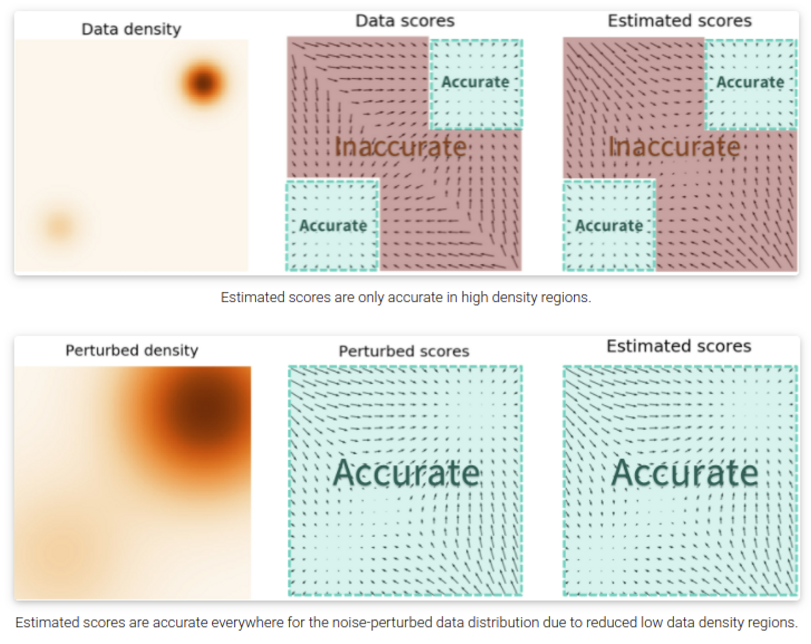
noise를 넣는것이 도움이 된다는 것은 이해가 되었으나 얼마나 noise를 넣어야 할까? 너무 많은 noise는 데이터의 밀도가 낮은 영역에서 더 정확한 score estimation이 가능하지만 원본 데이터가 손상되어 실제 분포와 멀어지는 문제가 있으며, 너무 적은 데이터는 반대로 데이터 밀도가 낮은 영역에서 score estimation 정확도의 문제를 해결하지 못한다.
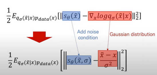
저자는 Generative Modeling by Estimating Gradients of the Data Distribution 논문에서 multiple scale noise perturbation을 사용하는 Noise Conditional Score Network(이하 NCSN)를 제시하였다 (위 식 참고). 매번 다양한 scale의 noise를 적용시키고 score function을 추정 후 loss를 계산하는 방식인데 code snippet과 함께 보면
# <https://github.com/ermongroup/ncsn>
sigmas = torch.tensor(
        np.exp(np.linspace(np.log(self.config.model.sigma_begin), np.log(self.config.model.sigma_end),
                           self.config.model.num_classes))).float().to(self.config.device)
for epoch in range(self.config.training.n_epochs):
    for i, (X, y) in enumerate(dataloader):
          step += 1
          score.train()
          X = X.to(self.config.device)
          X = X / 256. * 255. + torch.rand_like(X) / 256.
          if self.config.data.logit_transform:
              X = self.logit_transform(X)

          labels = torch.randint(0, len(sigmas), (X.shape[0],), device=X.device)
          if self.config.training.algo == 'dsm':
              loss = anneal_dsm_score_estimation(score, X, labels, sigmas, self.config.training.anneal_power)

def anneal_dsm_score_estimation(scorenet, samples, labels, sigmas, anneal_power=2.):
    used_sigmas = sigmas[labels].view(samples.shape[0], *([1] * len(samples.shape[1:])))
    perturbed_samples = samples + torch.randn_like(samples) * used_sigmas
    target = - 1 / (used_sigmas ** 2) * (perturbed_samples - samples)
    scores = scorenet(perturbed_samples, labels)
    target = target.view(target.shape[0], -1)
    scores = scores.view(scores.shape[0], -1)
    loss = 1 / 2. * ((scores - target) ** 2).sum(dim=-1) * used_sigmas.squeeze() ** anneal_power

    return loss.mean(dim=0)
최소, 최대 sigma 값을 설정하고 num_classes개의 sigma를 일정한 구간을 가지도록 뽑고 매 step마다 랜덤으로 scale을 sampling하고 해당 scale의 noise로 원본 데이터 X를 perturb한다.
score network가 유추한 score와 실제 score(위 식을 사용하여 구한)로 loss를 계산하여 score net을 update하는 것을 볼 수 있다.
Annealed Langevin Dynamics
샘플링은 noise scale을 점점 줄여가며 (우측 → 좌측) 단계별로 샘플링하는 Annealed Langevin Dynamics를 사용한다. (자세한 내용은 NCSN 논문 참고)
저자는 NCSN의 성공 요인을 multiple noise scale라고 분석하였으며 NCSN에서 discrete한 N(코드에서 num_classes)개의 noise scale을 continuous하게 확장하는 연구를 진행하였다.
noise scale이 continuous라고 하면 이는 Stochastic Differential Equations(SDE) 프레임워크로 설명이 가능해진다.
Stochastic Differential Equations(SDE)
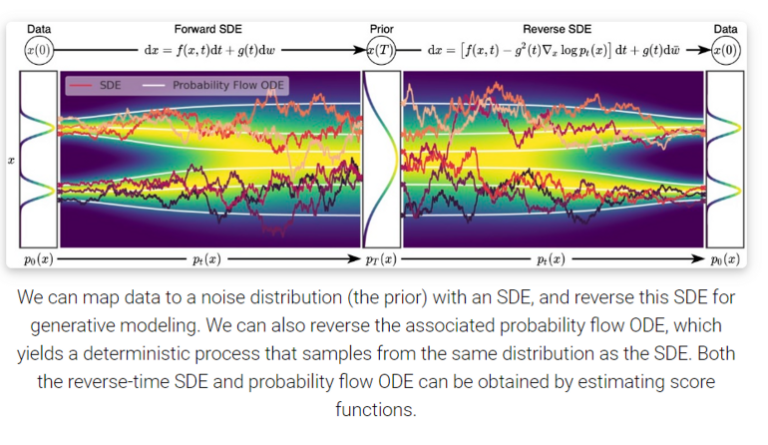
forward SDE는 아래 식의 형태로 표현할 수 있다.

$f(x,t)$ 는 drift coefficient, $g(t)$ 는 diffusion coefficient로 불리며 $w$ 는 standard Brownian motion, $dw$ 는 Infinitesimal white noise라고 불린다.
우변의 첫째항은 전체적인 추세를 나타내는 Drift, 둘째항은 Stochastic을 담당하는 Diffusion term으로 Diffusion term을 제외하고 보면 ODE의 형태를 보인다.
ODE는 하나의 초기값과 Drift coefficient가 주어지면 numerical하게 각 t에서 x가 결정되지만 SDE는 각 t에서 x가 random variable의 형태로 SDE를 푼다는 것은 모든 t에서 x의 marginal probability density function $p_t(x)$ 를 구하는 것을 말한다.
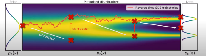
data에 multiple scale noise를 적용시키면, $p_0(x)$ 는 perturbation이 적용되지 않은 원본 데이터의 pdf이며 $p_T(x)$ 는 가장 많이 noise에 의해 perturb되어 prior distribution인 tractable한 noise distribution $\pi(x)$ 와 매우 유사해진다.
noise scale의 수가 무한이 됨에 따라 이제 연속적으로 noise를 적용시킬 수 있게 되었다. (아래 gif 참고)

먼저 noise scale이 무한해지고 따라서 SDE 프레임워크로 이를 다룰 수 있게 되어 생긴 이점을 나열해 보면 다음과 같다.
- multiple scale noise의 장점이 극대화되어 고품질의 샘플 생성
- SDE에 대응되는 ODE가 있어 전통적인 ODE Solver를 사용하여 빠른 sampling
- 기존 score-based model에서는 gradient인 score에 대한 근사만 하는 implicit model이나 SDE, ODE에서는 정확한 log-likelihood 계산이 가능
- inverse problem solving을 위한 controllable generation
- DDPM, Score-based generative model도 SDE 프레임워크로 설명 가능
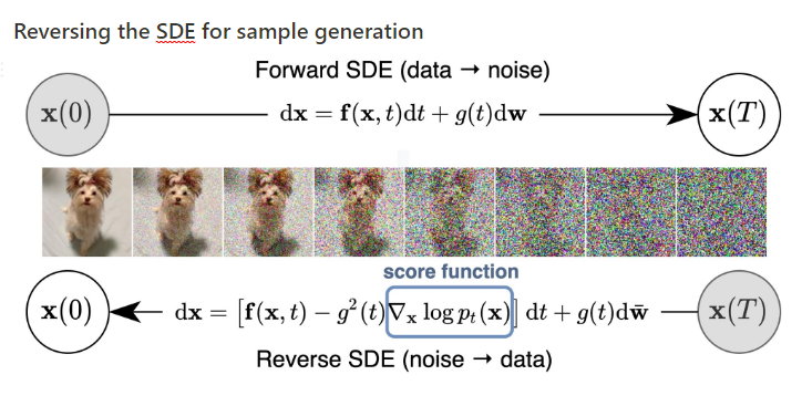
모든 forward SDE는 대응하는 reverse SDE가 존재한다 (Anderson 1982)

앞에서 forward SDE를 정의할 때 사용하는 term들이 모두 등장하고 추가로 $\nabla_x\log p_t(x)$ 가 reverse SDE 수식에서 등장하는데 이는 Score-based generative model에서의 score와 동일하다.
따라서 score를 추정하는 score network를 사용하여 score를 모델의 추정값 $s_\theta(x,t)$로 대체하여 reverse SDE를 풀 수 있다.
SDE의 numerical solver를 사용할 수 있는데 가장 간단한 Euler-Maruyama method를 사용해 보자.
0에 가까운 음수의 time step $\Delta t$ 를 정의하고 t를 T로 initialize하고 아래 과정을 t가 0에 가까워질 때까지 반복한다. ($z \sim N(0,1))$
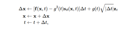
Milstein method, stochatic Runge-Kutta method 처럼 다른 SDE solver 또한 사용가능하다.
Predictor-Corrector Sampling
time-dependent score-based model $s_\theta(x,t)$ 를 통해 score를 추정하였고, 샘플링 과정에서는 각 timestep의 marginal distribution $p_t(x)$ 가 꼭 reverse SDE에서 샘플링된 특정 trajectory를 따르지 않아도 되기 때문에 $p_t(x)$ 를 추가로 변형시키는 것이 가능하다.
따라서 numercial SDE solver를 사용하여 얻은 trajectories를 MCMC를 사용하여 fine-tune 하여도 무방하다.
저자는 이를 논문에서 Predictor-Corrector Sampling이라는 표현으로 제시하는데 Numerical SDE Solver는 Predictor, predictor를 사용하여 얻은 trajectory를 score-function만 사용하여 추가로 fine-tune하는 Score-based MCMC를 Corrector라고 할 수 있다.
Predictor-Corrector 관점으로 이전 연구들을 보면 Score matching Langevin dynamics(SMLD)은 Predictor가 Identity, Corrector가 Annealed Langevin dynamics라고 볼 수 있으며 DDPM은 Predictor가 Ancestral sampling, Corrector가 Identity로 볼 수 있다.
Results

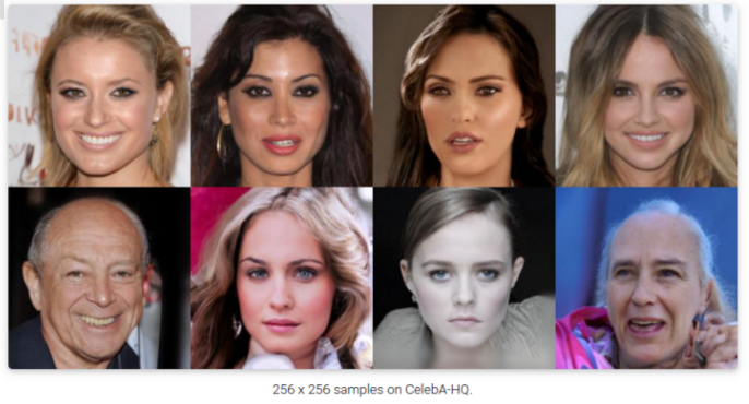
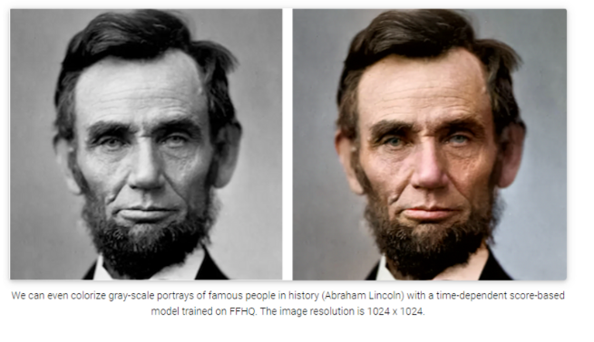
best GAN 모델인 StyleGAN2+ADA를 CIFAR-10 데이터셋에서 FID, IS 모두 넘어서며 SOTA를 달성하였고 1024 resolution의 고품질 이미지 생성 또한 성공하였다.
VE, VP SDEs
SDE에서 noise를 주는 방식은 hand-designed로 직접 정할 수 있는데
SMLD에서 noise를 입히는 perturbation kernel $p_{\sigma_i}(x|x_0)$ 은 아래 discrete Markov chain의 꼴로 정의된다.
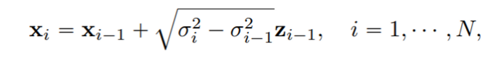
noise scale이 continuous하게 되어 무한히 많아지면 아래 SDE 꼴로 표현이 가능하다.
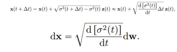
SMLD는 SDE의 discretization 관점으로 볼 수 있으며 위 식을 보면 SDE에서 Drift term이 없이 Diffusion term만 있으며 t가 커지게 되면 noise의 variance도 점점 커지는 Variance Exploding의 성질을 가지고 있어 VE-SDE이다.
마찬가지로 DDPM도 noise scale을 continuous하게 바꾸며 식을 전개한다. (Appendix 참고)

DDPM은 variance preserving의 성질을 가지는 VP-SDE라고 할 수 있다.
VE SDE는 t가 무한으로 커질 때, variance가 항상 explode 하는데 반해 VP SDE는 bounded variance이며 $p(x(0))$ 가 unit variance를 가지고 있으면 0 이상의 모든 t에서 constant unit variance를 유지한다.
Probability flow ODE
SDE Solver와 MCMC를 사용하여 퀄리티 높은 샘플을 생성할 수 있게 되었지만 log-likelihood를 정확하게 계산할 방법이 없다. 저자는 log-likelihood를 계산할 수 있는 sampler 기반 ordinary differential equations(ODE)를 제시한다.
논문에서는 marginal distribution $\{p_t(x)\}_{t\in[0,T]}$ 동일하게 유지한 채로 SDE를 ODE로 바꿀 수 있으며 이는 ODE를 풀어도 reverse SDE와 같은 분포에서 샘플링이 가능하다는 것을 말한다. (자세한 내용은 논문 참고)
SDE에 상응하는 ODE를 Probability flow ODE라고 하며 수식은 아래와 같고 reverse SDE와 마찬가지로 score function을 추정하여 식을 풀 수 있다.
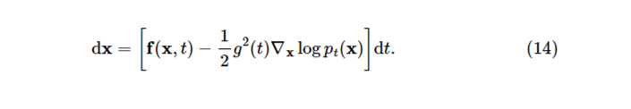
Probability flow ODE를 풀 때 score $\nabla_x\log p_t(x)$ 에 score network로 추정한 값 $s_\theta(x,t)$ 를 사용하는데 이는 ODE를 neural net으로 푸는 neural ODE의 special case로 볼 수 있다.
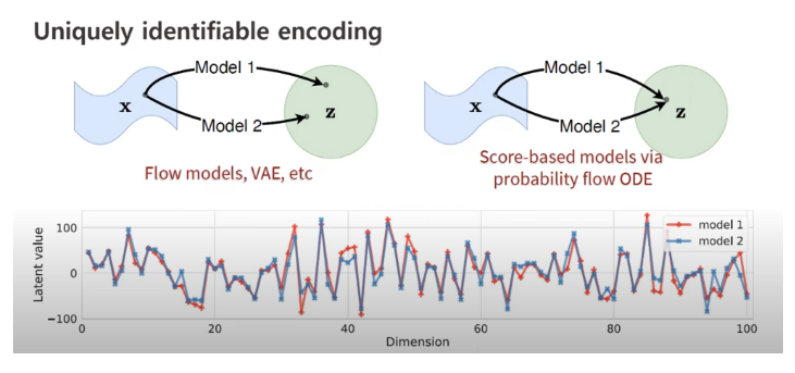
또 Probability flow ODE는 data distribution $p_0(x)$ 를 prior noise distribution $p_T(x)$ 로 전환시키고 (SDE의 marginal distribution을 공유하므로) invertible 하다는 점에서 normalizing flow 관점으로 볼 수도 있다.
ODE Solver는 score function evaluation 횟수(NFE) 측면에서 SDE Solver보다 효율적이라는 장점이 있다. (SDE Solver에서 1000 NFE 기준 샘플 퀄리티가 ODE Solver에서 100 NFE 기준 샘플 퀄리티와 비슷)
추가로 논문에서 Probability flow ODE는 이론/실험적으로 data와 latent가 unique하게 identify 된다고 하였다. (controllability, interpolation에서의 장점)
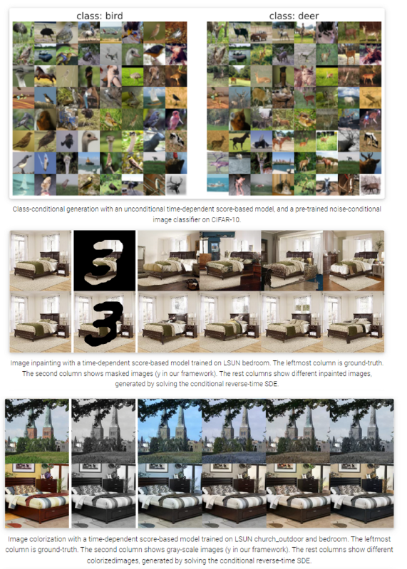
Controllable generation for inverse problem solving
Score-based model은 inverse problem을 풀기에 적합하다.
$x,y$ 가 random variable이고 $x$ 에서 $y$ 를 generate하는 forward process $p(y|x)$를 알고 있다고 가정해 보자. inverse problem은 $p(x|y)$ 를 계산하는 것인데, Bayes Rule을 적용시켜 보면 아래와 같다.
$$ p(x|y) = \frac{p(x)p(y|x)}{\int p(x)p(y|x)dx} $$
양변에 log를 씌우고 $x$ 에 대해 미분해 주면 식이 매우 간단해진다.
$$ \nabla_x\log p(x|y) = \nabla_x\log p(x)+\nabla_x\log p(y|x) $$
score matching으로 unconditional 데이터 분포의 score function을 추정하는 score network를 학습시키면 $s_\theta(x) \approx \nabla_x \log p(x)$ , forward process $p(y|x)$ 는 알고 있기 때문에 쉽게 posterior score function $\nabla_x\log p(x|y)$ 를 구할 수 있고 Langevin-type sampling을 통해 샘플 생성 또한 가능하다.
정리 & 후기
- Score function을 사용하는 이유, Score network를 사용하여 Score를 추정하기 위한 score matching 등 score-based generative model에 대한 배경지식에 대해 다루었다.
- multiple scale(discrete) noise를 continuous하게 변경하고 SDE의 관점으로 Score-based 모델을 바라보아 SDE Solver 사용, Probability flow ODE로의 변환을 가능하게 함
- SMLD, DDPM도 variance의 explode, preserving에 따라 VE-SDE, VP-SDE로 SDE 관점으로 해석이 가능함
- SDE의 marginal distribution을 공유하는 대응되는 ODE가 존재하고 ODE Solver로 이를 풀 수 있음 (Probability flow ODE)
- score-based model은 inverse problem을 풀기에 적합하며 condition forward process 모델이 있으면 쉽게 posterior score function를 구할 수 있다
Reference
[0] Yang Song et al, (2020), “Score-Based Generative Modeling through Stochastic Differential Equations”, https://arxiv.org/abs/2011.13456
[1] Generative Modeling by Estimating Gradients of the Data Distribution (Yang Song) https://yang-song.net/blog/2021/score/
[2] PR-400: Score-based Generative Modeling Through Stochastic Differential Equations (Jaejun Yoo) https://www.youtube.com/watch?v=uG2ceFnUeQU
'AI > Deep Learning' 카테고리의 다른 글
| Chain-of-Thought Prompting Elicits Reasoning in Large Language Models (0) | 2024.07.26 |
|---|---|
| LDM: High-Resolution Image Synthesis with Latent Diffusion Models (0) | 2023.06.02 |
| Score-based Generative Models과 Diffusion Probabilistic Models과의 관계 (0) | 2023.05.16 |
| Diffusion Models Beat GANs on Image Synthesis (0) | 2023.05.05 |
| Improved-DDPM: Improved Denoising Diffusion Probabilistic Models (0) | 2023.04.19 |


